Vector search explained: embeddings, indexes, distance metrics
Vector search turns text or images into lists of numbers and finds the stored lists closest to the query’s. The choices that matter are the distance measure (use the one your embedding model was trained for), the index (HNSW for most workloads, IVF or a disk-based index when memory is the limit) and how far you compress the vectors. Each trades recall for speed or memory, and only a test on your own data tells you how much.
What an embedding is
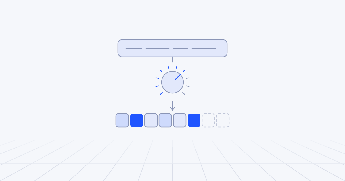
An embedding model reads a piece of content, such as a paragraph, a product description or an image, and outputs a fixed-length list of numbers: usually several hundred to a few thousand of them. The model is trained so that content with similar meaning produces lists that sit close together when you treat them as points in space. Embed the query with the same model, find the nearest stored points, and you have search by meaning.
Two things follow. The individual numbers mean nothing by themselves, and only distances between vectors carry information. And vectors from different models live in different spaces, so they cannot be compared or mixed in one index. We cover the model decision in choosing an embedding model. This article assumes you have vectors and need to store, index and search them.
Cosine, dot product or Euclidean: does it matter?
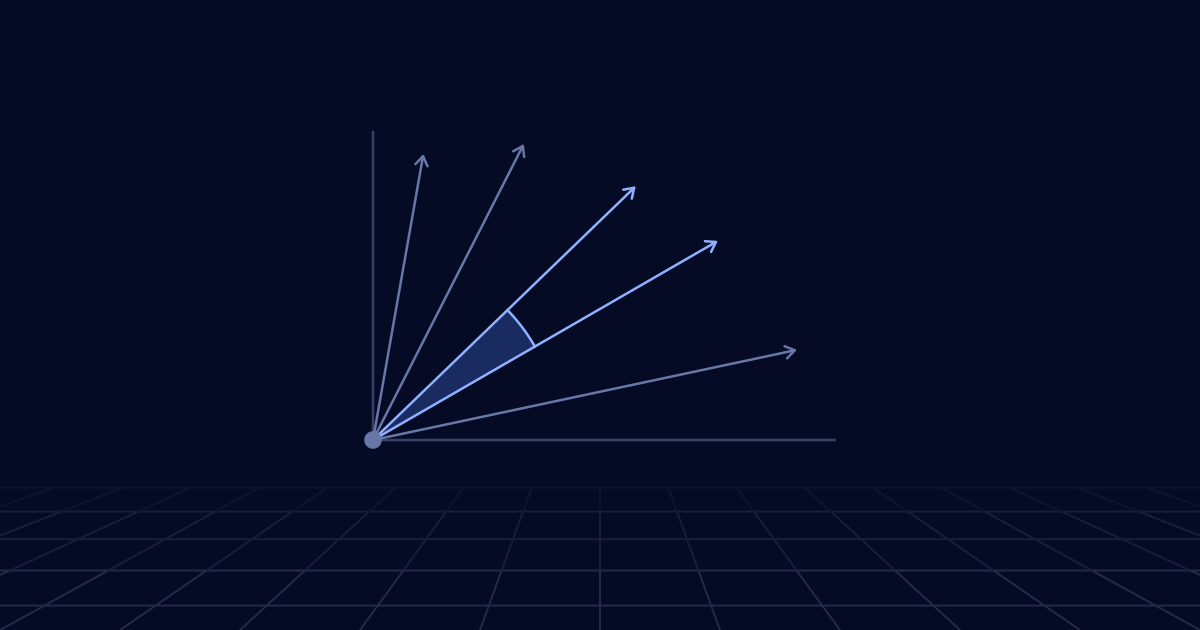
There are three common ways to measure closeness. Cosine similarity compares the angle between two vectors and ignores their length. Dot product, also called inner product, multiplies angle and length together. Euclidean distance, or L2, is the straight-line distance between the two points.
For vectors normalised to length 1, all three produce the same ranking, and many text embedding APIs return normalised vectors. OpenAI’s embeddings guide says so of its own models and adds that the choice of function then matters little, with dot product the cheapest to compute. The pgvector README gives the matching advice: for normalised vectors, use inner product for the best performance. Elasticsearch normalises vectors itself when you choose cosine, so that it can use dot product internally.
The choice matters in three situations.
- The model does not normalise. Then the length of a vector can carry signal, and the measures disagree. Use the one named on the model card. A wrong guess costs quality without raising any error.
- You shorten or compress vectors yourself. A truncated vector is no longer length 1. Re-normalise it, or cosine and dot product will stop agreeing.
- The index is built for one measure. In pgvector an index serves one distance operator. Query with a different one and Postgres falls back to scanning every row without telling you.
Exact versus approximate search
Exact search compares the query with every stored vector. It returns the true nearest neighbours every time. pgvector does this by default when no index exists, and its README describes the result as perfect recall.
The cost grows in a straight line with the collection. For a few tens of thousands of vectors it is fast enough that nobody notices. The same is true of a large collection when a filter narrows each query to a few thousand rows first. Plenty of systems that run an approximate index do not need one.
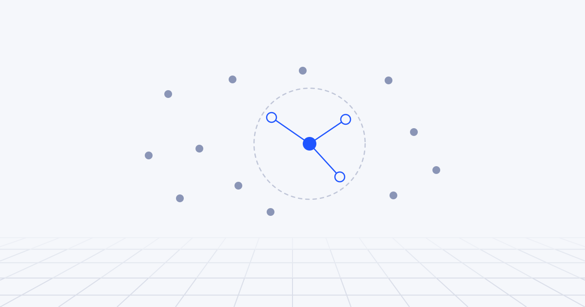
Approximate nearest-neighbour search, ANN, looks at a small fraction of the vectors and accepts that it will sometimes miss a true neighbour. The measure of that loss is recall: of the true top ten, how many came back. Every index below is a different way of deciding which fraction to look at.
How do HNSW and IVF indexes work?
HNSW: a graph you walk
HNSW (hierarchical navigable small world) links each vector to its nearest neighbours, forming a graph. The graph has layers. The top layer holds a few vectors with long links, like a motorway map. The bottom layer holds every vector, like a street map. A search enters at the top, moves greedily towards the query, drops down a layer and repeats. Malkov and Yashunin’s 2016 paper introducing it showed search cost growing logarithmically with the size of the collection, which goes a long way to explain why it is the usual default.
It has three knobs:
m: links per node. More links mean better recall, more memory and slower builds. The default is 16 in pgvector, Qdrant and Elasticsearch.ef_construction: how many candidates are considered when a vector is inserted. Higher builds a better graph more slowly. The default is 64 in pgvector and 100 in Qdrant and Elasticsearch.ef_search: how many candidates are kept during a query. This is the one to tune first, because it changes at query time with no rebuild. pgvector’s default is 40.
What it costs: the graph wants to sit in memory, builds are slow on large tables, and deleted vectors leave gaps that maintenance has to clean up.
IVF: clusters you probe
An inverted file index, IVF, groups the vectors into clusters and stores each vector in the list for its nearest cluster centre. A query finds the few nearest centres and scans only their lists.
It has two knobs. lists is the number of clusters: pgvector suggests rows divided by 1,000 for up to a million rows and the square root of the row count beyond that. probes is how many lists a query scans. pgvector’s default is 1, its suggested starting point is the square root of lists, and setting it equal to lists gives you exact search again.
IVF builds faster and uses less memory than HNSW, and gives lower recall for the same speed. It has to be built after the data is loaded, because the clusters are learned from the data. As the data shifts the clusters go stale, and the index needs rebuilding.
Index types side by side
| Index | How it searches | Memory | Build | Fits when |
|---|---|---|---|---|
| Flat (exact) | Compares with every vector | Vectors only | None | Small collections, very selective filters, ground truth for tests |
| IVF | Scans the nearest clusters | Low overhead | Fast, needs data first | Memory is tight and data changes slowly |
| HNSW | Walks a layered neighbour graph | High: vectors plus graph | Slow | Most workloads that fit in RAM |
| IVF or HNSW with quantisation | The same, over compressed vectors, then rescoring | Much lower | Similar | Tens of millions of vectors and more |
| Disk-based graph (DiskANN) | Graph on SSD, compressed vectors in RAM | Low | Slow | Collections larger than memory |
The last row is the newest in common use. The Milvus index guide describes DiskANN as a graph stored on disk with compressed vectors, and recommends it when the raw data sits on SSD.
Quantisation: smaller vectors, lower recall
Each number in a vector is normally a 32-bit float, 4 bytes. A 1,536-dimension vector is about 6 KB, and ten million of them are about 61 GB before any index. Quantisation stores each vector in fewer bits.
Scalar quantisation turns each float into an 8-bit integer, a fourfold saving. Qdrant’s quantisation guide puts the error it introduces at usually under 1%. Half-precision floats, which pgvector offers as halfvec, are a milder version that halves the size.
Binary quantisation keeps one bit per dimension, a 32-fold saving, and compares vectors with very fast bit operations. It throws away most of each vector, so it suits long vectors and needs a second pass over the originals. Qdrant’s guide restricts it to high-dimensional models and reports weak results on a 512-dimension one.
Product quantisation cuts each vector into chunks and replaces each chunk with the ID of the nearest entry in a learned codebook. It compresses furthest (Qdrant quotes up to 64 times) and is the slowest and least accurate of the three. Use it when memory is the only thing that matters.
What makes aggressive compression usable is rescoring. Search the compressed vectors for several times more candidates than you need, then re-rank those few against the full-precision originals kept on disk. Most of the lost recall comes back. This is now mainstream: Elasticsearch quantises new float vector fields by default, with its binary scheme applied to vectors of 384 dimensions and more since version 9.1, and puts the memory saving at 75% for 8-bit and about 96% for binary.
Why is metadata filtering hard?
Real queries carry filters: this tenant, this language, in stock. An ANN index is built on distance alone and knows nothing about them. There are three ways to combine the two, and each fails somewhere.
Filter after the search. Ask the index for the nearest 40 and drop those that fail the filter. The pgvector README gives the arithmetic: with its default settings and a filter matching 10% of rows, about four results survive on average. Since version 0.8.0 pgvector can keep scanning until enough rows pass, which fixes the count at some cost in speed.
Filter before the search. Find the matching rows with an ordinary index and compare them exactly. Recall is perfect. It is quick when the filter is selective and slow when it matches millions of rows.
Filter inside the index. Qdrant’s indexing documentation describes adding extra graph links based on indexed payload fields so that a search can stay within the matching vectors, with a planner that chooses between the payload index, the graph and a full scan. Those links are built only for payload indexes that already exist, so create the indexes before loading data. Version 1.16 added a method that looks at neighbours of neighbours when the direct ones are filtered out, at some cost in speed.
Take a parts catalogue with five million descriptions and the query “seal kit for hydraulic pump”, filtered to one brand and to items in stock. If the filter matches 2% of rows, filtering afterwards leaves less than one result from a top 40, while an exact search over the 100,000 matching rows works well. If the filter matches 60%, the opposite holds. Same data, same query, opposite answers. Know how selective your filters are before you choose an approach.
Measuring recall and latency on your own data
Published benchmarks use other people’s vectors and no filters. Measure your own.
- Take a few hundred real queries, with the filters they really carry.
- Compute the true neighbours for each with exact search. In pgvector, switch off index scans for that query. Other stores have an exact-search flag.
- Run the same queries through the index. Recall at k is the overlap with the true top k, averaged over queries.
- Record median and 95th-percentile latency at realistic concurrency, not one query at a time.
- Sweep the query-time knob (
ef_searchorprobes), plot recall against latency, and pick the point where the curve flattens. - Repeat with quantisation switched on, and again when the collection has doubled.
What we see go wrong most often is tuning on unfiltered queries and shipping filtered ones. The second most common is never measuring again. Recall drifts as data grows and nothing raises an error.
One caution on what this number means. A recall of 0.99 against exact search says the index is faithful to the embeddings. It says nothing about whether the right passage was among the true neighbours. That depends on the model and the chunking, and you measure it with labelled queries, as we describe in hybrid search and reranking.
Where to start
In the first week, load a real sample and run exact search with your real filters. Find out whether you need an approximate index at all.
If you do, start with HNSW at its defaults and raise ef_search until recall at 10 reaches your target. We usually aim for 0.95 or better. Reach for scalar quantisation with rescoring when the memory bill starts to hurt, and for anything more aggressive only with measurements in hand.
The first decision is where the vectors live, which we work through in vector database or pgvector. Building and tuning this layer is part of the vector search and data engineering we do at WeStack AI, usually as the retrieval half of a RAG system.